Predicting Spends with Sales – One line that fits them all

In the previous article we defined base sales as the consistent, ongoing sales a brand would achieve without any additional marketing efforts. Incremental sales, on the other hand, are the sales generated because of specific marketing campaigns or promotions.

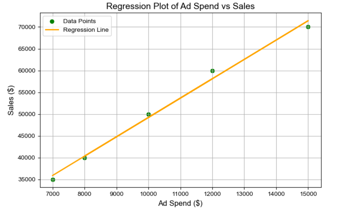
We then delved into how simple regression analysis can help separate base sales from incremental sales by plotting sales data against marketing spend. The intercept of the regression line represents base sales, while the slope represents the sales generated for each additional unit of marketing spend.

By analysing this relationship, brands can better understand their return on ad spend (ROAS) and the effectiveness of their campaigns in driving incremental sales. This approach helps optimize marketing strategies by focusing on maximizing the ROI from their marketing investments.

What are we trying to do?

In this article we will go through on how to find this intercept of the regression line which represents base sales, while the slope represents the sales generated for each additional unit of marketing spend.

How can we find this line?

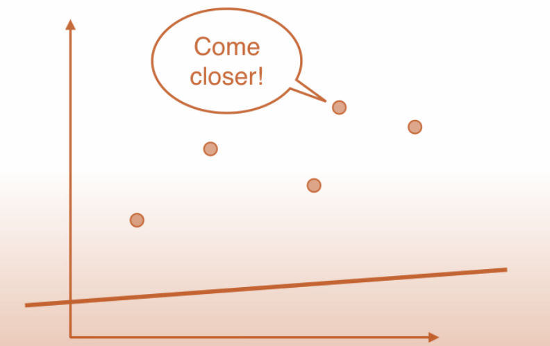
Essentially, we’re trying to find a line that gets as close as possible to all the data points. Think of it like a trial-and-error exercise—or rather, an iterative process—where we experiment with different combinations of the intercept (B0​) and slope (B1​), creating countless lines. In fact, there are infinite possibilities!

But don’t worry, we won’t be drawing an infinite number of lines manually. There’s a systematic process for finding that perfect line, especially in simple linear regression. It’s a bit more straightforward here compared to more complex algorithms, which we’ll explore later.

 

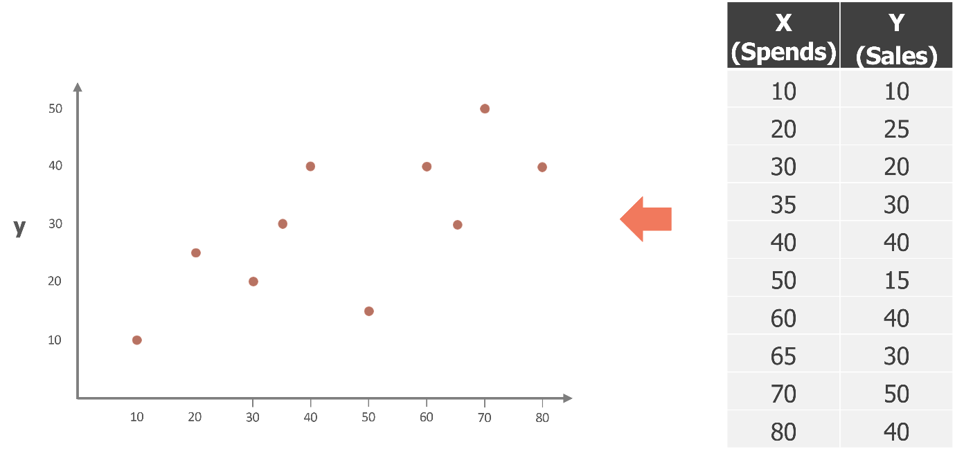
For now let’s break down how we find that line of best fit using a different dataset to make it easier to understand. Imagine we have some data points, as shown in the table on the right, where X represents the input variables (like ad spends), and Y represents the target variable (like sales). The green dots you see are the actual data points.

First Iteration

Now, if you’re asked to draw a line, the simplest place to start is to think of a line that represents the average value of all the Y points—essentially, the average sales. Imagine if you know nothing about X, like having no media spend data, and you only have the sales figures for the past few months. A reasonable starting point for predicting the next month’s sales would be to take the average of these figures and use that as your estimate.

This approach gives you a baseline—a simple average—represented by the black line in the chart. It’s a good initial guess and a straightforward way to begin thinking about a model.

However, here’s where it gets interesting. If you add up all the errors from this line, specifically the squared errors (because we’re using the Least Squares method), you’re calculating how far off your predictions are from the actual data points. If you do the math, summing the squared differences between each green dot (actual sales) and the black line (average sales), you get a total error of 1,450. 

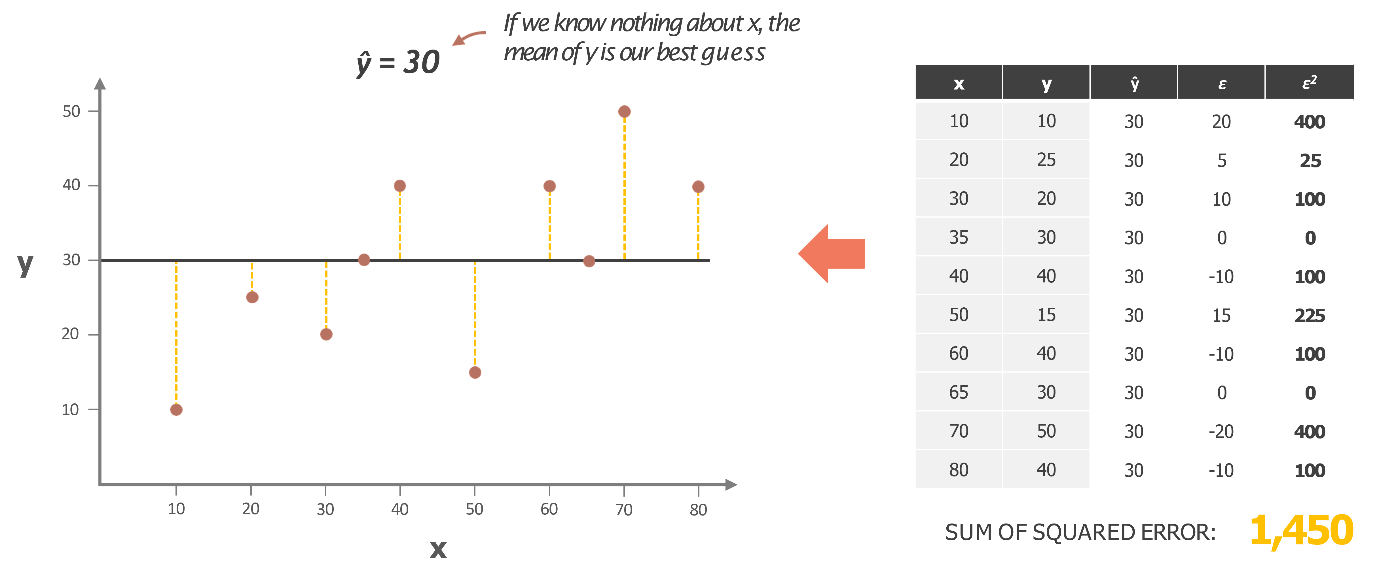
This sum of squared errors, also known as the Least Squares Error, tells us how well—or not—this simple average line fits the data. The goal now is to improve on this, reducing the error by finding a line that fits even better. This is just the starting point in our journey to build a more accurate regression model.

Second Iteration

Now, let’s tweak our line a bit. We adjust the angle, bringing the line closer to the data points—almost hugging them tighter. This gives us a new line with a different intercept, let’s say 10, and a different slope, say 0.5.

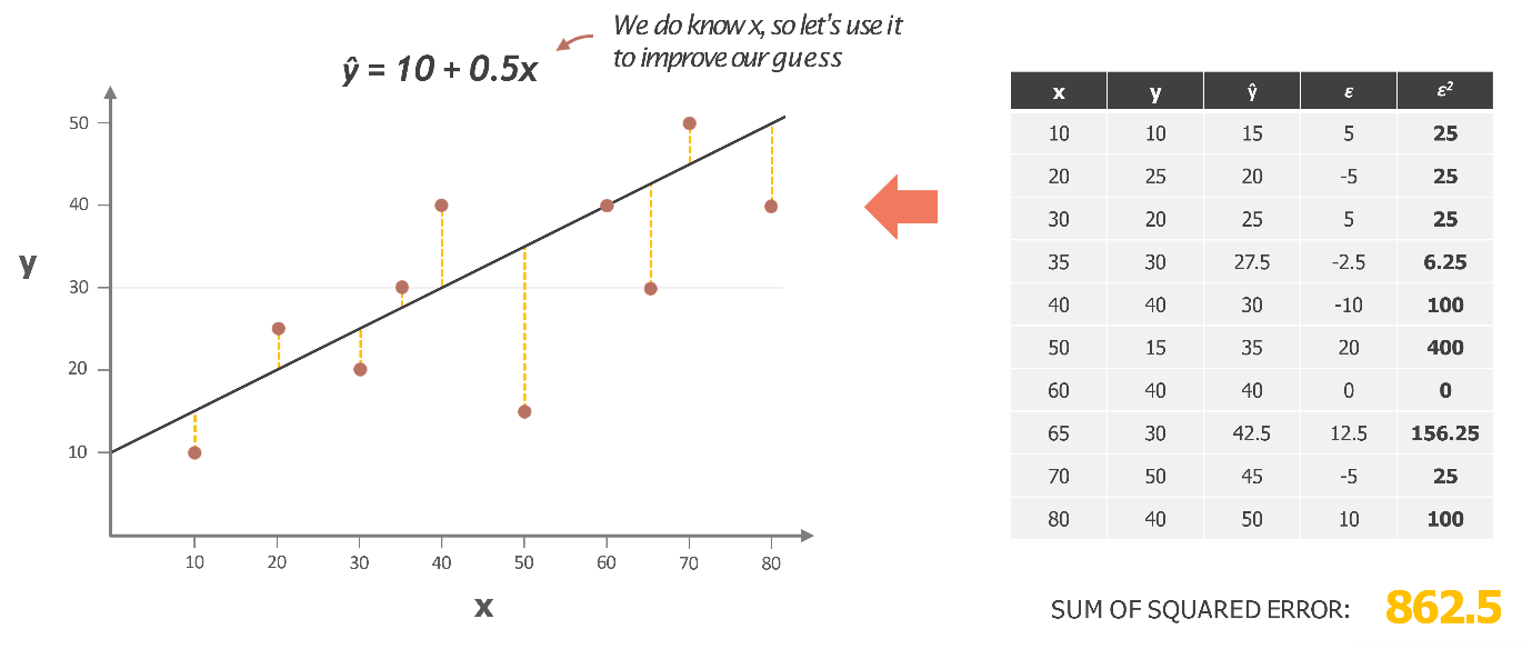
With this new line, we recalculate our predictions for Y based on the same X values. Because our line has changed, the predictions for each X value also change. And with these new predictions, we now have different errors—represented by the differences between the actual Y values and the predicted Y values. These errors are denoted by epsilon (ε).

To measure how well this new line fits, we square these errors (just like before) and sum them up to get the new sum of squared errors. This sum represents the total error for this new line.

So, what we’re doing here is comparing how much this new line improves (or maybe doesn’t improve) our model by checking if the sum of squared errors is lower than before. The goal is to find the line that minimizes this sum, giving us the best possible fit for the data. Keep this process in mind as it’s central to refining our regression model!

Third Iteration

You might have noticed that in our previous iteration, the sum of squared errors was lower compared to when we just used the average of Y for all predictions. This time, we refined the line even further. We realized it was a bit too far from some points, so we adjusted by reducing the slope slightly. Now, we have a new line with an intercept of 12 and a slope of 0.4.

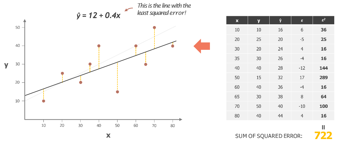
After recalculating with these new values, you can see that the overall error, or the total sum of squared errors, has dropped to 72—this is the lowest we’ve seen across the three scenarios. Clearly, if we had to choose from these three lines, this line would be our pick, as it fits the data best. It serves as the strongest model out of the three we’ve discussed.

But here’s the million-dollar question: does the process stop here? How do we know if we’ve truly found the best regression line, the one that can’t be improved any further with the current variables and inputs?

There could still be room for improvement, and it’s crucial to explore how to ensure our model is the best possible representation of the relationship between our variables.

General process to find the best model

This brings us to a fundamental set of steps that aren’t just limited to simple linear regression; they lie at the heart of nearly every machine learning algorithm. Now, we won’t dive deep into the specifics of what all machine learning algorithms are, but if you’re even a bit familiar with the current landscape of artificial intelligence and machine learning, you know that most advances in predictive sciences are rooted in these steps.

By the very name “machine learning,” we’re talking about machines learning something—and what they learn is how to reduce errors with each iteration. That’s exactly what we just did when we looked at the three different lines: with each iteration, we tried to reduce the overall error.

Here’s a formalized 4-step process that encapsulates this concept:

1. Start with a Hypothesis: We began with a simple hypothesis that our model could be represented by a straight line, like Y=β0+β1. Here, β0 ​ is the intercept, and β1 is the slope of the line. This is the initial assumption about the relationship between the variables.
2. Define the Parameters: Next, we identified the parameters we’re trying to fine-tune: β0. These are the variables we adjust to find the best possible model.
3. Represent the Error with a Cost Function: A critical aspect of this process is having a representation of the error—what’s often called the cost function. Rather than just calling it error, because we squared the differences between the actual values and the predicted values (to keep them positive and emphasize larger errors), it’s referred to as a “cost function.” This is essentially the cost of making incorrect predictions—the larger the error, the higher the cost.
4. Minimize the Cost Function: Finally, the goal is to minimize this cost function. In the language of machine learning, this function is often denoted by J. Our objective is to find the values of β0​ that minimize J. By finding this minimum, we arrive at our optimal model.

These four steps are not just specific to regression; they are universal across all machine learning algorithms, whether it’s deep learning, advanced machine learning models, or ensemble techniques. At the core, all these models work by iterating through these steps: starting with a hypothesis, defining the parameters, using a cost function to measure error, and iteratively minimizing that error to find the best model. This process of optimization is what allows machines to “learn” and refine their predictions.

In the next article we will discuss how to make sure we have been able to minimize the model as much as possible with the help of a technique called ‘Gradient Descent Method’.